Imagine you’re trying to evaluate multiple AI agents on a battery of tests, but you can’t observe all agent-item pairs due to computational constraints. How do you infer the missing performance data? We’ll review total variation distance (TVD) and mutual information (MI) and how it can be connected with the Rasch model in item response theory (IRT) using the principle of maximum entropy. This sparse evaluation problem led me to use information theory through maximum entropy to make a precise solution that is naturally compatible with how TVD-MI works. We then validate assumptions and show how it can reduce the sampling requirements to estimate TVD-MI.

Information Elicitation. The basic TVD–MI definition leads to an formulation of the information elicitation problem that can be applied to black-box agents. We emphasize the Rasch model applies to the TVD-MI metric calculation, but the agents themselves give free-responses. In this way we can apply IRT without ground-truth labels. Let \(P^+ := P_{XY}\) denote the joint distribution of paired responses (same source) and \(P^- := P_X \otimes P_Y\) denote the product of marginals (independent sources). Following the \(f\)-divergence framework of Csiszár (1974) the TVD mutual information between a pair of agent response random variables \((X;Y)\) can be written as:

where \(\text{TV}(P, Q) = \frac{1}{2}\|P - Q\|_1\) is the total variation distance.

This choice is motivated by several key advantages. First, TVD offers direct interpretability as it measures the maximum difference in probability assignments, making it immediately interpretable as a discrimination advantage. Second, the computational tractability of TVD-MI has been demonstrated by Robertson & Koyejo (2025), who show it can be naturally evaluated with an LLM judge framework through binary classification items. Finally, TVD provides robustness since it is bounded and less sensitive to rare events than KL divergence.

Variational Estimation. The metric implementation requires modeling the distributions, which is impractical when we only have black-box interaction protocols with agents. However, for total variation distance, we can introduce an overseer agent who has a reasoning map \(r : \mathcal{T}(S) \to \mathcal{C}\) which can be applied to the empirical joint type of a sample \(S\) from responding agents. Formally we have a definition for the empirical type.

Definition: (Empirical Joint Type) Given a sample \(S=\{(x_1,y_1),\dots,(x_N,y_N)\}\), let \(\mathcal{T}(S)(a,b)\) be the number of occurrences of pair \((a,b)\) in \(S\). The empirical joint type is the contingency table \(\mathcal{T}(S)\) modulo independent permutations of the row and column labels. Any estimator depending only on this statistic is called type-based.

With acceptance set \(A \subseteq \mathcal{C}\) we have the variational identity (Tsybakov, 2008, Definition 2.4) which tells us

Restricting to a type-based decision \(r\), define

Then, by data processing,

This shows us that we can estimate lower-bounds for TVD-MI by carefully aggregating classifications across a positive and negative set of data derived from the agent response.

The Sparse Evaluation Problem. Suppose we have \(k\) agents to evaluate over \(n\) items. The number of MI pairs to be evaluated would be \(\tfrac{1}{2} k \cdot (k-1)\), and within each evaluation we would have at least \(2n\) evaluations if we want to estimate using the variational bound. Is there a way to do the evaluation with sparse data?

Our basic variables will be \(z_{ij} \in \lbrace -1, 0, +1 \rbrace\) which indicate for agent \(i \in [k]\) whether the classification for item \(j\) they completed was classified accurately on the “true positive” set, accurately on the “true negative” set, or contributed nothing as the overseer made an inaccurate classification contributing zero to the variational bound.

To build intuition, suppose we have the full agent-item dataset. We have \((Y_1, \ldots, Y_k)\) for the agent response distributions, we have \(S_{ij}\) for each agent-item pair, and then the agent sum scores satisfy the following relation:

This can be calculated from data and it can be used to produce agent evaluations without ground truth, i.e., mutual information is robust to agents that obfuscate information by DPI.

So our goal is to recover probabilities \((p_{ij}^+, p_{ij}^0, p_{ij}^-)\) for the agent-item statistics without necessarily evaluating all the pairs. To simplify the derivation, we observe that false positive rates are negligible: agents rarely claim to detect signal when none is present. We drop true negative instances \(z_{ij} = -1\) from our data accordingly and model \(p_{ij}\) for binary outcomes.

Shannon MaxEnt to Rasch Model. Here is the formal setup for our recovery problem:

1. Observations. We obtain data \(\mathcal{D} = \lbrace z_{ij} \rbrace_{(i,j) \in I}\) where \(I\) is a multi-set of agent-item indices.
2. Processing. We then calculate moments \(g_{ij} = \mathbb{E}[z_{ij}]\) along the subset \(\text{set}(I)\) (eliminate repeats in the multi-set).
3. Inference: We model the moments with \(p_{ij}\) on the full agent-item domain.

So now we can write down our inference program. We maximize (pairwise independent) entropy:

subject to the following constraints for all \((i,j) \in \text{set}(I)\):

Observational Consistency. We enforce \(p_{ij} = g_{ij}\)

Item Independence. Across rectangles \((i,i', j, j')\) we have:

where \(\ell\) is a link function, here \(\ell = \text{logit}\). The item independence assumption is strong as we see below.

Lemma (Discrete Integrability — 1PL Case). The system of rectangle constraints above has feasible solutions if and only if there exist parameters \(\theta_i, b_j \in \mathbb{R}\) such that:

That is, the link-transformed responses admit an additive decomposition into agent ability and item difficulty.

Proof. First we show sufficiency. Suppose the rectangle constraints hold for all \((i,i',j,j')\). Fix a reference pair \((i_0,j_0)\). Define:

Then, for any \((i,j)\), we have:

by the rectangle identity. Hence \(\ell(g_{ij}) = \theta_i - b_j\). Now we show necessity. If \(\ell(g_{ij}) = \theta_i - b_j\), then:

so the rectangle constraints hold. □

However, this yields precisely the Rasch model from item response theory (Rasch, 1993), where \(\theta_i\) represents the ability of agent \(i\) and \(b_j\) serves as the difficulty parameter for item \(j\).

In practice, what tends to happen is that people instead optimize the dual of the program above which is known to be equivalent to MLE and is easier to obtain feasible solutions to as it is effectively an unconstrained optimization problem. So why didn’t we just start with the MLE formulation?

The Saturation Problem. The logistic model works well when \(g_{ij}\) stays away from the boundaries. However, in the TVD-MI framework, good discriminative tests naturally produce saturation. When high-quality agents encounter easy items where \(\theta_i \gg b_j\), we expect \(g_{ij} \to 1\). This leads to logit explosion, as \(\text{logit}(g_{ij}) \to \infty\) when \(g_{ij} \to 1\), causing numerical instability where standard optimization becomes ill-conditioned near boundaries unless regularization is introduced.

This is not a bug but a feature of TVD-MI: saturation indicates perfect discrimination. The challenge is that the logistic link function is fundamentally incompatible with boundary behavior, it maps the entire real line to \((0,1)\), never reaching the boundaries.

The empirical reality is that many agent-item pairs will saturate. Expert agents consistently solve easy items, yielding \(g_{ij} = 1\), while agents fooled by obfuscating agents on certain items would result in \(g_{ij} = 0\). Perhaps this is an artifact of using TVD-MI with binary scores. We want to expand our search for a saturation-aware alternative that respects the natural geometry of TVD-MI.

TVD-Ent Program. Instead of Shannon entropy, we consider the Gini index (also known as Rényi-2 entropy). In fact we have the following,

This is the natural entropy measure in the TVD framework for several reasons. Its quadratic form leads to computationally tractable optimization problems. It naturally handles boundary cases, achieving zero entropy at \(g \in \{0,1\}\), which aligns with our intuition about certainty. So overall it mirrors \(I_{\text{KL}}(g;g) = \text{Ent}(g)\) and maintains theoretical coherence throughout our framework.

To simplify the optimization formulation and make the quadratic structure more apparent, we’ll work with the centered score which allows us to write in compact form

Now we can express the TVD-Ent program in primal form.

To derive the dual, we can calculate the convex conjugate of \(s_{ij}^2\) with the condition it’s less than one from which we obtain the Huber loss,

So we leave the constraint implicit in \(s_{ij} - t_{ij} = (\theta_i - b_j) - t_{ij}\) so we may apply the method of Lagrange multipliers to obtain:

Here we can interchange max and min because the primal problem is convex with a strictly feasible point (Slater’s condition), ensuring strong duality holds. Finally, we can enforce unconstrained optimization on the manifold and obtain:

So now we have defined two ways to approach the (Rasch) matrix factorization. One uses the maximum Shannon entropy principle. The other uses a generalized maximum TVD entropy principle.

Experimental Validation. We validate the curl-free assumption and test how well we can implement sparse sampling TVD-MI comparisons from 30 agents generating new article summaries (xSum benchmark). Two diagnostics are used.

Curl-free validation. We test discrete integrability of the empirical matrix by computing the average violation of the curl-free constraint

The mean absolute violation across 20,000 random rectangles was 0.25, with 90th percentile ≈ 0.53, confirming moderate but recoverable deviations from a perfect Rasch manifold. This supports that the 1PL (Rasch) factorization is a plausible approximation.

Sparse sampling study. We fitted the additive Rasch model \(s_{ij} = \theta_i - b_j\) under structured sparsity patterns and evaluated hold-out RMSE. Dense training yields RMSE ≈ 0.102. Under row/column subsampling, accuracy remains near-dense (RMSE ≈ 0.107–0.111) down to ~0.24 coverage. We also try to look at going from the default \(O(k^2)\) scaling with \(k\) agents to \(O(k \log k)\) scaling. We achieve near-dense accuracy with 3-4 fewer observations (RMSE 0.107 at ≈28% coverage, 0.128 at ≈14% coverage). Below ~0.08 coverage, connectivity breaks and test RMSE increases sharply.

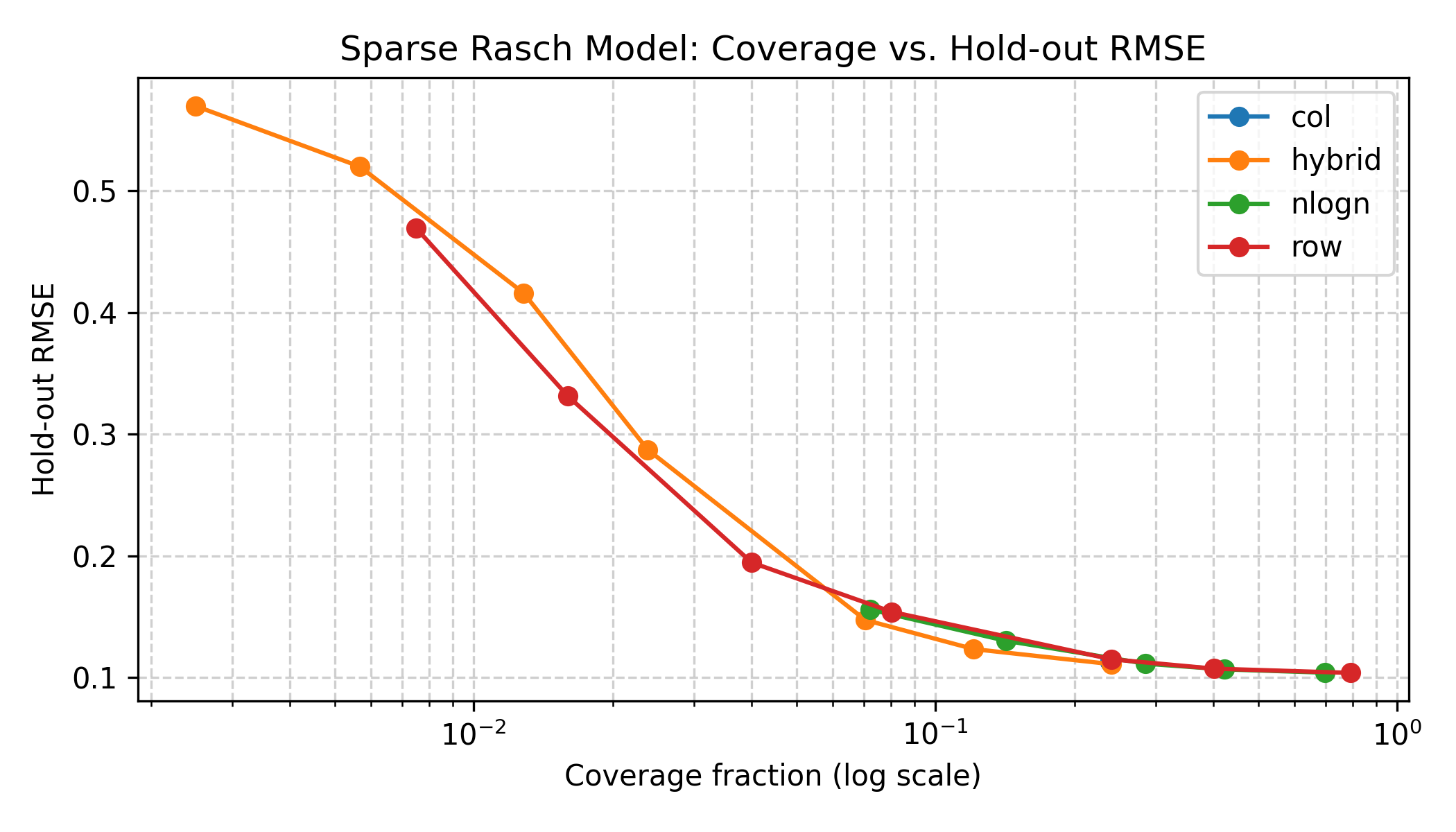
Figure 1: Sparsity vs Hold-Out RMSE. A log-x plot showing coverage fraction on the x-axis and hold-out RMSE on the y-axis. Include separate curves for Row, Column, Hybrid, and \(n\log n\) regimes. Highlight the efficient frontier around 0.23–0.28 coverage where RMSE ≈ 0.11.

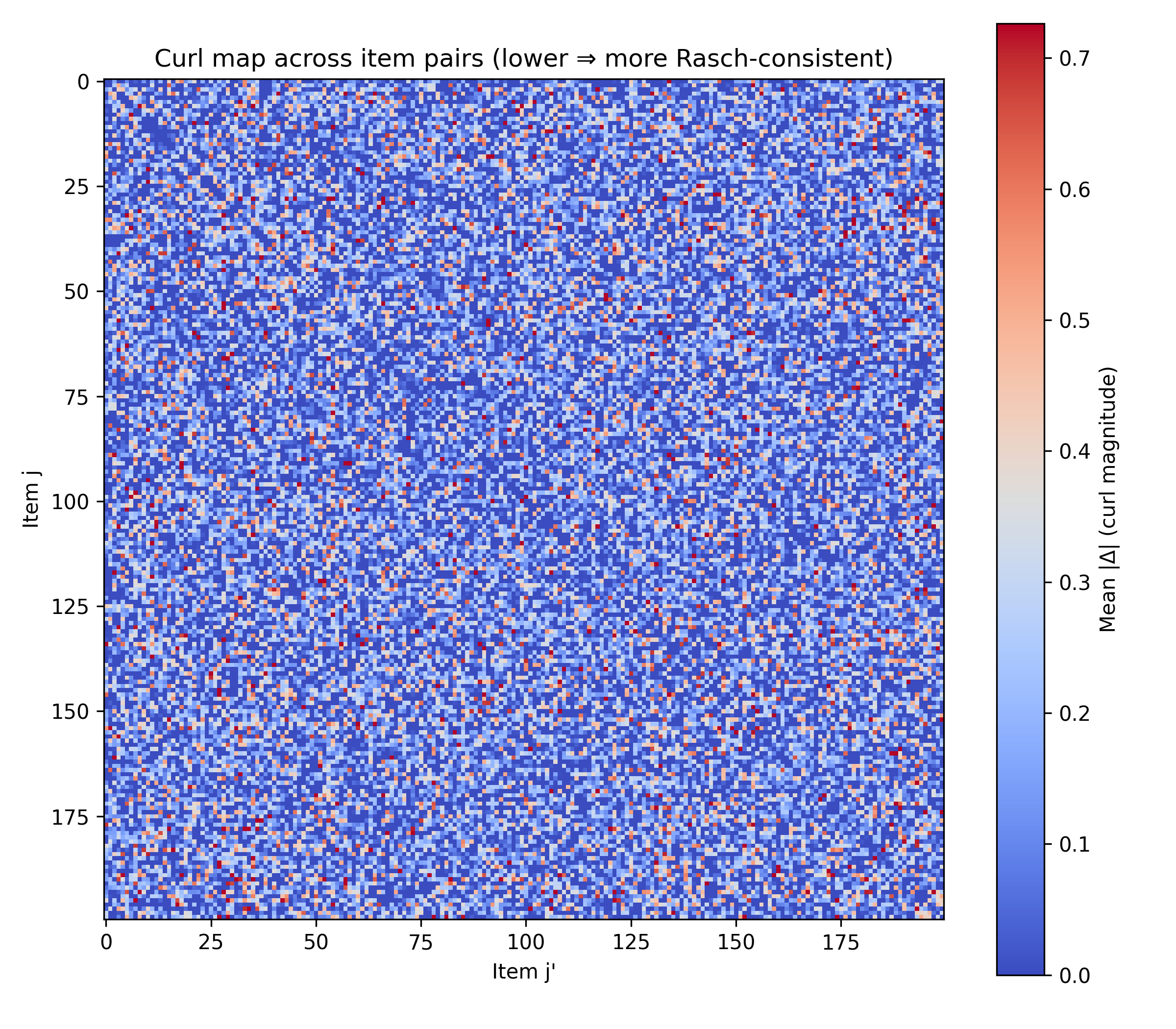
Figure 2: Curl-Free Violation Distribution. Histogram (or boxplot) of rectangle deviations. The bulk near 0.2–0.3 with a tail > 1 illustrates that while the empirical surface is not perfectly integrable, it is sufficiently close for Rasch-style decomposition to capture the dominant structure.

Together these plots demonstrate that the maximum entropy formulation admits a Rasch-like low-rank structure, and that sparse evaluation can reproduce full-information estimates efficiently.

If this was useful to you, please consider citing.

@misc{robertson2025humans,
  title={From TVD Mutual Information to Item Response Theory - Clipped-Linear Alternative to Logistic Models},
  author={Robertson, Zachary},
  year={2025},
  month={October},
  institution={Stanford University},
  url={https://zrobertson466920.github.io/TVDRasch/},
  note={Blog post relating TVD mutual information with IRT}
}

References

Csiszár, I. (1974). Information measures: A critical survey. In Transactions of the Seventh Prague Conference on Information Theory, Statistical Decision Functions, Random Processes (pp. 73-86).

Mead, L. R., & Papanicolaou, N. (1984). Maximum entropy in the problem of moments. Journal of Mathematical Physics, 25(8), 2404-2417.

Rasch, G. (1993). Probabilistic models for some intelligence and attainment tests. ERIC.

Robertson, Z., & Koyejo, S. (2025). Let’s Measure Information Step-by-Step: LLM-Based Evaluation Beyond Vibes. arXiv preprint arXiv:2508.05469.

Tsybakov, A. B. (2008). Nonparametric estimators. In Introduction to Nonparametric Estimation (pp. 1-76). Springer.